Introduction to BGE-M3
Key features and performance of the model
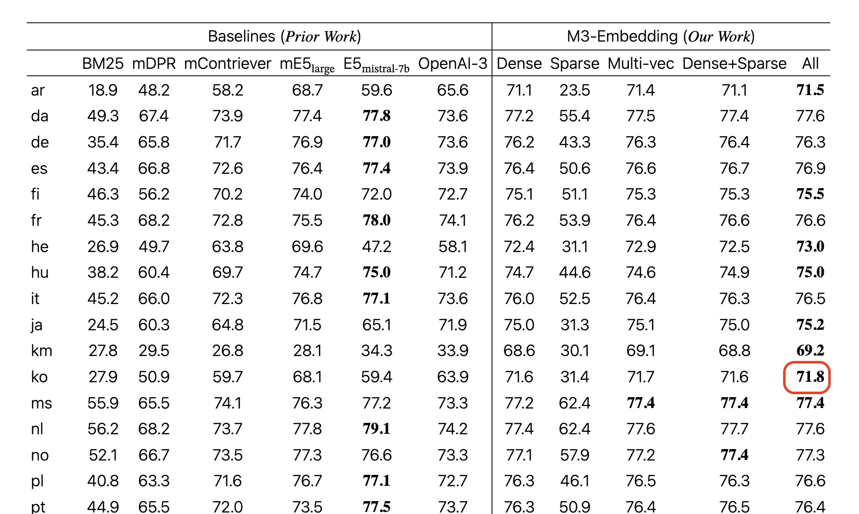
Source : https://arxiv.org/html/2402.03216v3 Cross-lingual retrieval performance on MKQA (by Recall@100)
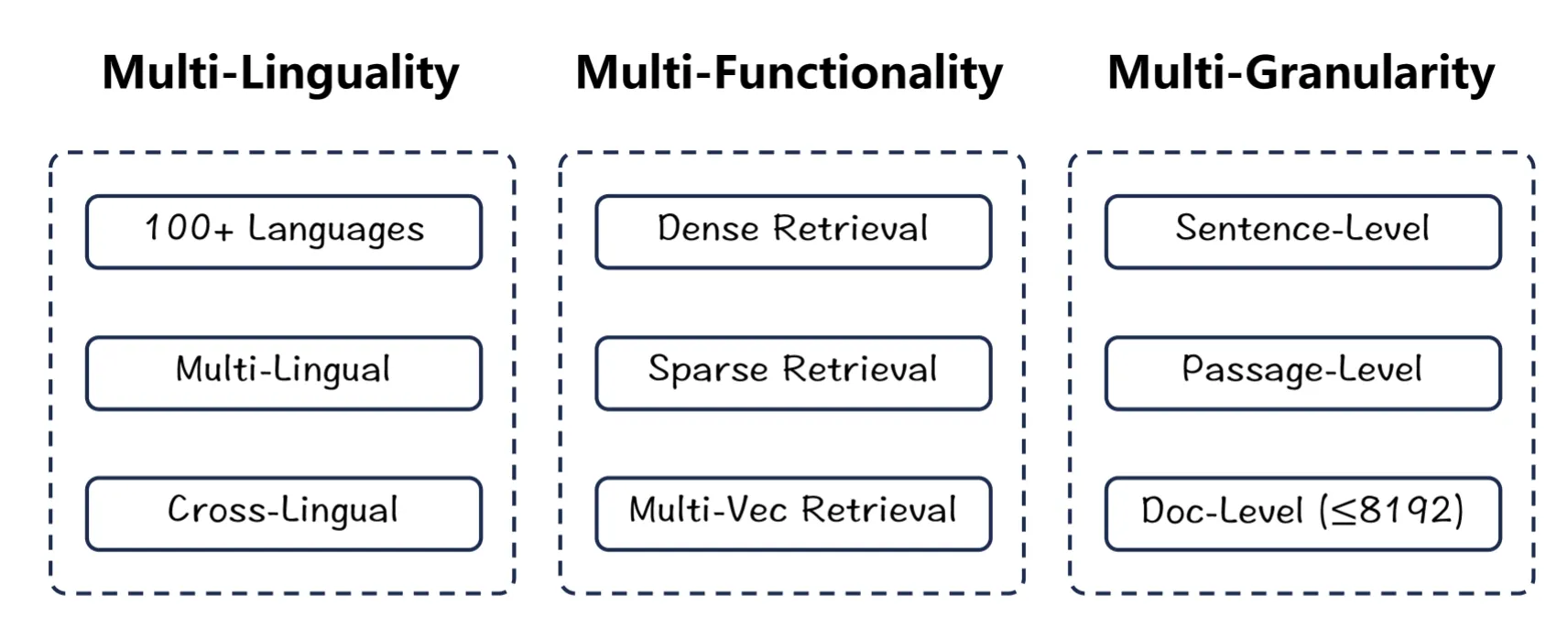
BGE-M3 is a multilingual embedding model that supports over 70 languages. It has a rich multilingual vocabulary consisting of approximately 250,000 tokens and shows particularly outstanding performance in Korean.
In the MTEB (Massive Text Embedding Benchmark) Korean benchmark, it achieved top-level performance compared to existing multilingual embedding models, particularly in retrieval and classification tasks. Notably, it delivers competitive results against Korean monolingual embedding models while retaining the advantage of multilingual support.
For these reasons, BGE-M3 has recently become one of the most frequently used models in vector retrieval tasks through embedding vector extraction, such as in RAG (Retrieval-Augmented Generation).
Three Retrieval Loss Function Structures
BGE-M3 model is characterized by simultaneously optimizing the following three retrieval loss functions:
1.
Dense Retrieval
•
Semantic search via sentence-level CLS vectors
•
Compresses and represents the meaning of entire sentences into a single vector
2.
Lexical Retrieval
•
Search via token-level importance weights
•
Improves keyword-based search performance by learning the importance of each token
3.
Multi-Vector Retrieval
•
Search via token-level vectors
•
Enables fine-grained semantic matching through independent vector representations for each token
Loss Functions in the Original Model Implementation
RoBERTa XL-based Architecture
Since XLMRobertaModel (link), which forms the basis of the model structure, is already a well-proven classic architecture, the inference model structure is very simple and clear disregarding the training-related techniques. For example, the following techniques commonly seen in recent Transformer models were not applied in this article:
•
Rotary Position Embedding (RoPE)
•
Pre Normalization
•
Linear bias removal
How to print the BGE-M3 model structure through the huggingface-transformers library
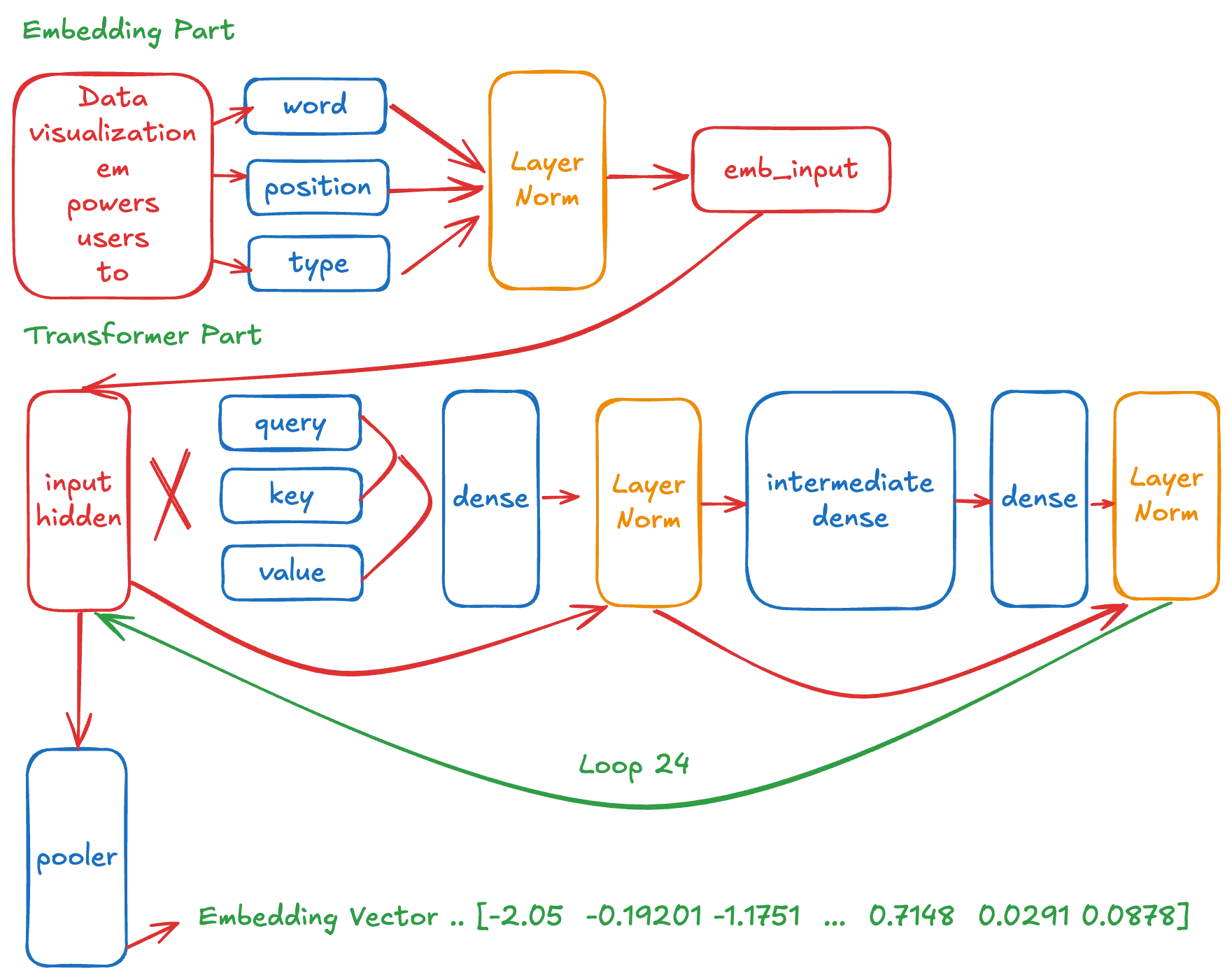
Thus, the model's inference structure can be almost perfectly implemented with just 9 basic linear Layers (Dense, Linear, MLP) and 3 LayerNormalization.
Figure 1 Schematic of the BGE-M3 model
Since it has a structure where Transformer blocks are repeated 24 times, you essentially only need to implement the following key layers:
•
3 embedding-related layers
•
9 layers within the Transformer block
•
3 LayerNormalization layers
By defining these basic components and their computational relationships, you can implement the complete inference structure of the BGE-M3 model.
TensorFlow - Keras Implementation
We introduce the Keras implementation as an example, which provides the easiest packaging for deployment and the most straightforward abstraction interface.
BGE-M3 Model Implementation
First, we define the basic model class.
class BGEM3TensorFlow(tf.keras.Model):
Scala
복사
Embedding Layer Implementation
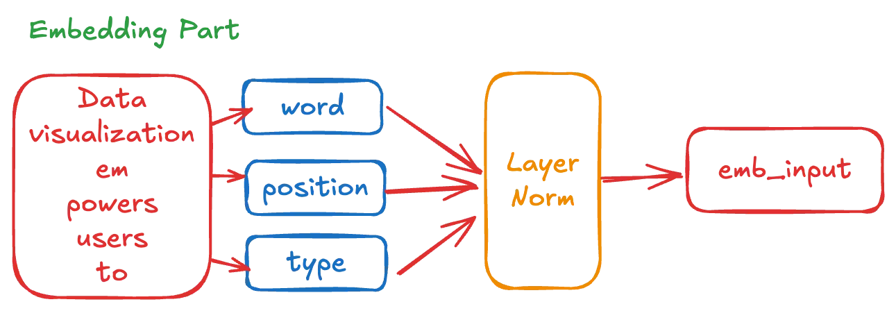
The embedding layer is a core component that converts natural language into numerical vectors that the model can understand. BGE-M3 uses three types of embeddings:
1.
Word Embedding
•
Vocabulary size: 250,002 tokens
•
1,024-dimensional vector representation per token
•
Example:
◦
A word with token ID 0 is mapped to the 0th row (1,024 dimensions) of the embedding table
◦
A word with token ID 5000 is mapped to the vector in the 5000th row
2.
Position Embedding
•
Size: 8,194 positions (8,192 + 2)
•
1,024-dimensional vector representation per position
•
Encodes position information of tokens in the sequence
3.
Token Type Embedding
•
Only uses a single type in BGE-M3
•
A fixed 1,024-dimensional vector applied equally to all tokens
•
Can be cached as a constant for performance optimization
The implementation of these embedding layers is as follows:
def __init__(self,...):
# Word embeddings
self.word_embedding = tf.keras.layers.Embedding(
input_dim=250002,
output_dim=1024,
)
# Position embeddings
self.position_embedding = tf.keras.layers.Embedding(
input_dim=8194,
output_dim=1024,
)
# Token type embeddings
self.token_type_embedding = tf.keras.layers.Embedding(
input_dim=1,
output_dim=1024,
)
# Layer normalization and dropout
self.layer_norm = tf.keras.layers.LayerNormalization(epsilon=1e-5)
#self.dropout = layers.Dropout(rate=0.1)
Python
복사
This embedding structure effectively converts text into numerical form at the model's input stage, transforming it into a format that subsequent Transformer layers can process. Among these, since token_type_embeddings only uses a single value, it can be replaced with a pre-calculated constant vector for performance optimization during inference.
Figure 2 Embedding Part
Using tf.gather, the numerical sequence of word tokens is converted into embedding tensors. They are then normalized by passing through the layerNorm layer.
def call(self, ..)
self.inputs_embeds = tf.gather(params=self.weight, indices=input_ids)
self.position_embeds = tf.gather(params=self.position_embeddings, indices=position_ids)
self.token_type_embeds = tf.gather(params=self.token_type_embeddings, indices=token_type_ids)
embedding_output = inputs_embeds + position_embeds + token_type_embeds
embedding_output = self.layerNorm(embedding_output)
Python
복사
Additional Information
With this implementation, the basic embedding part of the model is complete, and approximately 20% of the overall model structure can be considered implemented.
The next step requires the implementation of the Transformer Block, which is the core part of the model.
Transformer Block Structure
Figure 3 Transformer Block Part
Each Transformer Block consists of the following major components:
•
6 Dense layers
•
2 LayerNormalization layers
•
2 Residual computations
First, we define the base class.
class TransformerBlock(tf.keras.layers.Layer):
Scala
복사
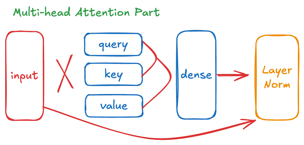
Looking at the weight structure of the original model above, the Mult-head Attention Part requires the following components:
Figure 3-1 Transformer Attention Part
1.
Multi-head Self-Attention Components
# Query, Key, Value weights
encoder.layer.0.attention.self.query | shape: torch.Size([1024, 1024])
encoder.layer.0.attention.self.key | shape: torch.Size([1024, 1024])
encoder.layer.0.attention.self.value| shape: torch.Size([1024, 1024])
# Attention output processing
encoder.layer.0.attention.output.dense | shape: torch.Size([1024, 1024])
encoder.layer.0.attention.output.LayerNorm | shape: torch.Size([1024])
Markdown
복사
2.
Multi-head Self-Attention Components
# Intermediate Layer
encoder.layer.0.intermediate.dense | shape: torch.Size([4096, 1024]) # expand
encoder.layer.0.output.dense | shape: torch.Size([1024, 4096]) # reduce
# Final Normalization
encoder.layer.0.output.LayerNorm | shape: torch.Size([1024])
Markdown
복사
Keras's default Multi-head Attention is based on 3D Attention and has some slight implementation differences. We will create a custom implementation of Multi-head Attention by referring to the structure of the huggingface official implementation.
def __init__(self, ...):
self.wq = tf.keras.layers.Dense(1024)
self.wk = tf.keras.layers.Dense(1024)
self.wv = tf.keras.layers.Dense(1024)
self.dense = tf.keras.layers.Dense(1024)
self.attlayerNorm = tf.keras.layers.LayerNormalization(epsilon=1e-5)
self.intermediate = tf.keras.layers.Dense(4096)
self.output_dense = tf.keras.layers.Dense(1024)
self.output_norm = tf.keras.layers.LayerNormalization(epsilon=1e-5)
Scala
복사
In this implementation, the Dropout layers used only during training can be omitted. The next section will cover how to connect these layers to implement the actual operation of a Transformer Block.
Multi-head Attention Implementation
def call(self, ..)
input = embedding_output
# Query, Key, Value를 계산
q = self.wq(input) # (batch_size, seq_len, d_model)
k = self.wk(input) # (batch_size, seq_len, d_model)
v = self.wv(input) # (batch_size, seq_len, d_model)
# 다중 헤드로 분리
q = self.split_heads(q, batch_size, 16, 64) # (batch_size, num_heads, seq_len_q, depth)
k = self.split_heads(k, batch_size, 16, 64) # (batch_size, num_heads, seq_len_k, depth)
v = self.split_heads(v, batch_size, 16, 64) # (batch_size, num_heads, seq_len_v, depth)
def split_heads(self, x, batch_size, num_heads, depth):
x = tf.reshape(x, (batch_size, -1, num_heads, depth))
return tf.transpose(x, perm=[0, 2, 1, 3]) # (batch_size, num_heads, seq_len, depth)
Python
복사
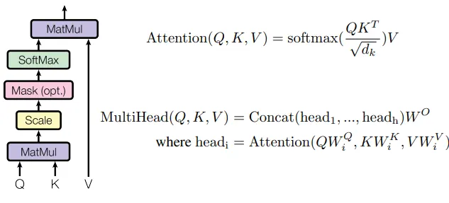
Q, K, V are calculated through the three dense layers defined in the model structure above.
Through a simple operation called split_heads, they are separated into the defined number of multi-heads.
Here we apply the Scaled Dot-Product Attention used by the XLM RoBERTa model.
This divides the attention_scores by 8.0, the dk value calculated for this model's scale.
Then multiplies by v again to obtain the final Attention result.
# Scaled Dot-Product Attention Score
dk = tf.cast(math.sqrt(1024 // 16), tf.float32)
attention_scores = tf.matmul(q, k, transpose_b=True) # (batch_size, num_heads, seq_len_q, seq_len_k)
attention_scores = tf.divide(attention_scores, dk)
attention_probs = tf.nn.softmax(attention_scores + 1e-9, axis=-1)
# Calculating the Attention Output
attention_output = tf.matmul(attention_probs, v) # (batch_size, num_heads, seq_len_q, depth)
attention_output = tf.transpose(attention_output,
perm=[0, 2, 1, 3]) # (batch_size, seq_len_q, num_heads, depth)
attention_output = tf.reshape(attention_output,
(batch_size, -1, self.d_model)) # (batch_size, seq_len_q, d_model)
# Passing Attention Output through the final Dense Layer
attention_output = self.dense(attention_output) # (batch_size, seq_len_q, d_model)
#attention_output = self.dropout(inputs=attention_output, training=training)
# First Residual Connection
attention_output = self.attlayerNorm(inputs=attention_output + input)
Python
복사
The final output value is obtained through a dense layer. The first residual connection is applied by adding the initial input embedding value or the hidden value from the previous layer block, followed by normalization.
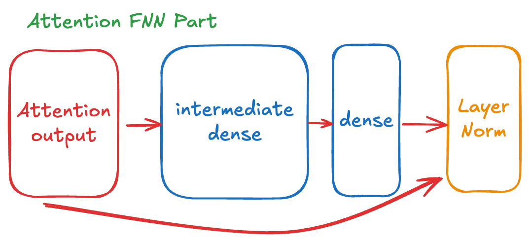
Transformer Feed-Forward Neural Network (FFN) Implementation
The following image shows the Feed-Forward Neural Network part, which is the second major component of the Transformer Block.
Figure 3-2 TransformerBlock FNN (FeedForward Neural Network) Part
# intermediate layer
intermediate_output = self.intermediate(attention_output)
intermediate_output = self.gelu_approx(intermediate_output) # Use exact GELU approximation
layer_output = self.output_dense(intermediate_output)
layer_output = self.output_dropout(layer_output, training=training)
# Second Residual Calculation
output = layer_output + attention_output
output = self.output_norm(output)
# GELU Approximation
def gelu_approx(self, x):
x = tf.convert_to_tensor(x)
cdf = 0.5 * (1.0 + tf.math.erf(x / tf.cast(tf.sqrt(2.0), x.dtype)))
return x * cdf
Python
복사
The input passes through an intermediate dense layer with a size four times larger than the hidden dimension of the basic output layer. The output from this dense layer is then added to the previous attention_output to perform the second residual connection, followed by normalization.
The BGE-M3 model basically repeats this structure 24 times.
encoder_layers = []
for i in range(self.num_layers):
layer = TransformerBlock(
d_model=1024,
num_heads=16,
intermediate_size=4096,
dropout_rate=self.dropout_rate,
name=f"encoder.layer.{i}"
)
encoder_layers.append(layer)
Python
복사
Since BGE-M3 explicitly skips the pooler layer, the implementation below can simply be left as a dummy.
pooler.dense.weight | shape: torch.Size([1024, 1024])
pooler.dense.bias | shape: torch.Size([1024])
Scala
복사
Model Forward Flow Summary
Token Embedding Process
def call(self, input_ids, ..)
inputs_embeds = tf.gather(params=self.weight, indices=input_ids)
input_shape = shape_list(inputs_embeds)[:-1]
position_ids = self.create_position_ids_from_input_ids(input_ids=input_ids))
position_embeds = tf.gather(params=self.position_embeddings, indices=position_ids)
token_type_ids = tf.fill(dims=input_shape, value=0)
token_type_embeds = tf.gather(params=self.token_type_embeddings, indices=token_type_ids)
embedding_output = inputs_embeds + position_embeds + token_type_embeds
embedding_output = self.layerNorm(embedding_output)
def create_position_ids_from_input_ids(self, input_ids, past_key_values_length=0, padding_idx=1):
mask = tf.cast(tf.math.not_equal(input_ids, padding_idx), dtype=input_ids.dtype)
incremental_indices = (tf.math.cumsum(mask, axis=1) + past_key_values_length) * mask
return incremental_indices + padding_idx
Python
복사
•
position_ids are generated through create_position_ids_from_input_ids, referring to the official implementation.
•
token_type_ids are all filled with 0.
•
Using tf.gather, converts the sequence of token indices into embedding tensors at corresponding positions.
•
Adds all three embeddings together and normalizes by passing through the layerNorm layer.
Processes the Attention Mask to be injected into the Transformer Block.
attention_mask_shape = shape_list(attention_mask)
extended_attention_mask = tf.reshape(
attention_mask, (attention_mask_shape[0], 1, 1, attention_mask_shape[1])
)
Python
복사
•
Reshapes the existing attention_mask to (batch_size, 1, 1, sequence_length) format.
•
This is a preparation process for broadcasting in multi-head Attention.
shape_list function format
extended_attention_mask = tf.cast(extended_attention_mask, dtype=embedding_output.dtype)
one_cst = tf.constant(1.0, dtype=embedding_output.dtype)
ten_thousand_cst = tf.constant(-10000.0, dtype=embedding_output.dtype)
Scala
복사
•
Explicitly converts the mask to the same data type as the embeddings.
•
Defines constants of 1.0 and -10000.0.
extended_attention_mask = tf.multiply(tf.subtract(one_cst, extended_attention_mask), ten_thousand_cst)
Python
복사
•
Performs the computation (1 - mask) * -10000.
•
In the original mask, 1 represents actual tokens, and 0 represents padding.
•
After this operation:
◦
Actual token positions (originally 1) → 0
◦
Padding positions (originally 0) → -10000
•
This processing makes the Attention scores of padding positions close to 0 during Softmax operation.
This outputs the final hidden_state after passing through 24 transformer blocks through the computation below.
# embedding_output = inputs_embeds + position_embeds + token_type_embeds
hidden_states = embedding_output
# Pass through encoder layers
for layer in self.encoder_layers:
hidden_states = layer(
hidden_states,
attention_mask=attention_mask,
)
Python
복사
BGE-M3's default vector output uses only the first vector per final hidden batch, which is the CLS token.
pooled_output = hidden_states[:, 0, :] # (batch, seq_len, hidden_dim)
Python
복사
For BGE-M3's multi-vector output, it must pass through one additional separate layer. Since the default huggingface's official XLMRobertaModel doesn't support this, separate weights need to be loaded and computed.
The model's structure and output values can be defined as follows:
self.colbert_linear = tf.keras.layers.Dense(
units=self.d_model,
)
colbert_vecs = self.colbert_linear(hidden_states[:, 1:])
colbert_vecs = colbert_vecs * tf.cast(attention_mask_origin[:, 1:][:, :, None], dtype=tf.float32)
Python
복사
The separate additional weights of the original model can be applied as follows.
Since the provided additional weights are in pytorch format, they need to be read through torch as follows.
model_path = "./bge-m3/colbert_linear.pt"
colbert_model = torch.load(model_path, map_location=device, weights_only=True)
colbert_weights = colbert_model['weight']
colbert_bias = colbert_model['bias']
tf_model.colbert_linear.set_weights([
colbert_weights.numpy().T,
colbert_bias.numpy()
])
Python
복사
The final embedding vector output of the model can be created as follows.
outputs = {
"dense_vecs": pooled_output, #[batch, hidden_size]
"colbert_vecs" : colbert_vecs, #[hidden, seq_len, hidden_size]
#"lexical_weights" : sparse_embedding,
}
return outputs
Python
복사
Model Signature Creation, Packaging and Saving
Additionally, you can save and package the final model with the following
def save_model_with_tokenizer(model, tokenizer, save_path):
"""Save both model and tokenizer"""
os.makedirs(save_path, exist_ok=True)
model_save_path = os.path.join(save_path, 'model')
# Ensure model is built by calling it with dummy inputs
dummy_inputs = {
'input_ids': tf.zeros((2, 11), dtype=tf.int32),
'attention_mask': tf.ones((2, 11), dtype=tf.int32)
}
_ = model(dummy_inputs, training=False, output_hidden_states=True)
# Define serving signature
@tf.function(input_signature=[
tf.TensorSpec(shape=[None, None], dtype=tf.int32, name='input_ids'),
tf.TensorSpec(shape=[None, None], dtype=tf.int32, name='attention_mask')
])
def serving_fn(input_ids, attention_mask):
print(input_ids)
inputs = {
'input_ids': input_ids,
'attention_mask': attention_mask
}
outputs = model(inputs=inputs, training=False)
return {
'dense_vecs': outputs['dense_vecs']
'colbert_vecs': outputs['colbert_vecs']
}
# Save model
tf.saved_model.save(
model,
model_save_path,
signatures={'serving_default': serving_fn}
)
# Save tokenizer
tokenizer.save_pretrained(save_path)
return model_save_path
Python
복사
Through the implementation and content above, you can secure a code base for model structures that can be deployed across almost all platforms, web, and mobile.
Usage Examples:
•
Large-scale hadoop-spark operations using tensorflow-java-scala
•
Federated learning and inference personalized RAG service using kotlin-springboot
•
Mobile and embedded inference using tensorflow-lite
•
Inference and custom implementation at Apple npu-gpu level using tensorflow-metal
Appendix
Model and Weight Conversion Code Examples
Converted Model Verification Results
Example Code


